บทความนี้จะใช้การ Record Macro และแก้ไข VBA Code เล็กน้อย เพื่อให้สามารถทำงานซ้ำๆ กับ Worksheet ที่มีรูปแบบเหมือนกัน ดาวน์โหลดไฟล์ได้ที่นี่

ขั้นตอนการทำงานแบบ Manual

ถ้าเราทำเองก็จะต้องทำงานต่างๆ เช่น เพิ่มบรรทัด 2 บรรทัด, เพิ่มคอลัมน์ Total, ใส่สูตร SUM(), เพิ่มคอลัมน์ Trend, ใส่ Line Sparklines, สร้างกราฟ, ใส่ชื่อ Report แล้วทำทุก Worksheet

ต้นฉบับ

สิ่งที่ต้องการ

สมมุติว่าทุก Worksheet มีข้อมูลเท่ากันทั้งจำนวน row และ column ก็จะสามารถใช้การ Record Macro ได้เลย

กด “Record Macro”

1. เพิ่มบรรทัด 2 บรรทัด
2. เพิ่มคอลัมน์ Total แล้วใส่สูตร SUM(), ใส่ Data Bars
3. เพิ่มคอลัมน์ Trend แล้วใส่ Line Sparklines
4. ตกแต่งตาราง เช่น auto fit, ใส่สี header, ทำตัวหนา, เปลี่ยนสีตัวอักษร, ตีเส้น
5. สร้างกราฟ Product กับ Total
6. ใส่คำว่า Weekly Report

กด “Stop Recording”

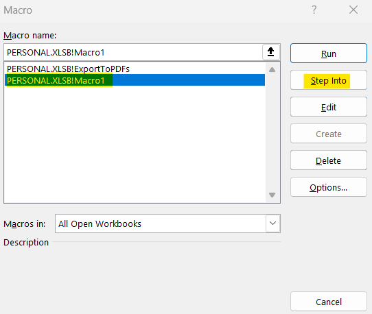
จากนั้นกด “Macros”

เลือกชื่อ Macros ที่เพิ่ง record ไป แล้วกด “Step Into”

จะมีหน้าต่าง Microsoft Visual Basic for Applications ขึ้นมา ให้เลื่อนไปช่วงท้ายๆ ของโค้ด แล้วลบชื่อของ Worksheet และสัญลักษณ์ ! ออกไป (ในที่นี้คือ Anna)

Code ที่ได้จากการ Record Macro

จัดระเบียบโค้ดด้วย ChatGPT

ให้ ChatGPT ช่วยใส่ comment (การเขียน prompt แบบด้านล่างนี้เรียกว่า Short prompt, Ready to run) สั่งให้ ChatGPT พร้อมรับงานในครั้งถัดๆ ไป โดยไม่ต้องทวนคำสั่งซ้ำ

I'll provide VBA code, and your task is add comment in it

ใส่ prompt แล้วรอ ChatGPT ตอบกลับมา แล้ววาง Code 1 ในแชท

ถ้าในอนาคตเราจะให้ ChatGPT ช่วยใส่ comment ให้ ก็มาวาง Code ลงในแชทที่เคยสั่งงานไว้ได้เลย กรณีนี้ลองใส่ Code อื่นลงไปในแชทเลย (ใช้ code ของคราวที่แล้ว)

Copy Code จาก ChatGPT ไปวางในหน้า Microsoft Visual Basic for Applications จะได้ code ที่มี comment และจัดระเบียบให้อ่านง่าย

R1C1 Reference Style

จากตัวอย่าง Record Macro ด้านบน อยากจะแนะนำวิธีการอ่านโค้ดให้สักเล็กน้อยเกี่ยวกับการอ้างอิงเซลล์

ตอนที่เราคลิกที่ cell J3 ใส่คำว่า Total แล้วคลิกที่ cell J4 เพื่อใส่สูตร SUM() ได้ code ออกมา ดังนี้

Range("J4").Select
ActiveCell.FormulaR1C1 = "=SUM(RC[-7]:RC[-1])"

Range(“J4”).Select คือ เลือก cell J4

ActiveCell.FormulaR1C1 = “=SUM(RC[-7]:RC[-1])” คือ การเขียนสูตร SUM() ใน cell ปัจจุบันที่เลือกอยู่ โดยใช้การอ้างอิงแบบ R1C1

R คือ row ปัจจุบันที่สูตรอยู่ C[-7] คือ column ก่อนหน้า 7 column (จะได้ cell C4)

R คือ row ปัจจุบันที่สูตรอยู่ C[-1] คือ column ก่อนหน้า 1 column (จะได้ cell I4)

ก็จะได้สูตร =SUM(C4:I4) นั่นเอง

Sub WeeklyReport()
'
' Macro1 Macro
'
' Keyboard Shortcut: Ctrl+Shift+Q
'
    ' Insert two new rows at the top
    Rows("1:2").Select
    Selection.Insert Shift:=xlDown, CopyOrigin:=xlFormatFromLeftOrAbove
    
    ' Add "Total" label in cell J3
    Range("J3").Select
    ActiveCell.FormulaR1C1 = "Total"
    
    ' Add SUM formula in cell J4, calculating the sum of values from column C to I
    Range("J4").Select
    ActiveCell.FormulaR1C1 = "=SUM(RC[-7]:RC[-1])"
    
    ' Autofill the SUM formula from J4 to J10
    Range("J4").Select
    Selection.AutoFill Destination:=Range("J4:J10")
    Range("J4:J10").Select
    
    ' Add "Trend" label in cell K3
    Range("K3").Select
    ActiveCell.FormulaR1C1 = "Trend"
    
    ' Maximize the Excel window
    Range("K4").Select
    Application.WindowState = xlMaximized
    Application.CutCopyMode = False
    Range("K4").Select
    
    ' Insert sparklines in column K for trend visualization (based on data in columns C to I)
    Range("$K$4").SparklineGroups.Add Type:=xlSparkLine, SourceData:="C4:I4"
    
    ' Set sparkline series and marker colors
    Selection.SparklineGroups.Item(1).SeriesColor.Color = 9592887
    Selection.SparklineGroups.Item(1).SeriesColor.TintAndShade = 0
    Selection.SparklineGroups.Item(1).Points.Negative.Color.Color = 208
    Selection.SparklineGroups.Item(1).Points.Negative.Color.TintAndShade = 0
    Selection.SparklineGroups.Item(1).Points.Markers.Color.Color = 208
    Selection.SparklineGroups.Item(1).Points.Markers.Color.TintAndShade = 0
    Selection.SparklineGroups.Item(1).Points.Highpoint.Color.Color = 208
    Selection.SparklineGroups.Item(1).Points.Highpoint.Color.TintAndShade = 0
    Selection.SparklineGroups.Item(1).Points.Lowpoint.Color.Color = 208
    Selection.SparklineGroups.Item(1).Points.Lowpoint.Color.TintAndShade = 0
    Selection.SparklineGroups.Item(1).Points.Firstpoint.Color.Color = 208
    Selection.SparklineGroups.Item(1).Points.Firstpoint.Color.TintAndShade = 0
    Selection.SparklineGroups.Item(1).Points.Lastpoint.Color.Color = 208
    Selection.SparklineGroups.Item(1).Points.Lastpoint.Color.TintAndShade = 0
    
    ' Autofill sparklines from K4 to K10
    Selection.AutoFill Destination:=Range("K4:K10"), Type:=xlFillDefault
    Range("K4:K10").Select
    
    ' Bold the text in row 3 (header row)
    Range("K3").Select
    Range(Selection, Selection.End(xlToLeft)).Select
    Selection.Font.Bold = True
    
    ' Auto-fit columns A to K
    Columns("A:K").Select
    Columns("A:K").EntireColumn.AutoFit
    
    ' Apply Currency format to the range C4:J10
    Range("C4:J10").Select
    Range("J4").Activate
    Selection.Style = "Currency"
    
    ' Apply background color to header row (A3:K3)
    Range("A3:K3").Select
    With Selection.Interior
        .pattern = xlSolid
        .PatternColorIndex = xlAutomatic
        .ThemeColor = xlThemeColorLight2
        .TintAndShade = 0
        .PatternTintAndShade = 0
    End With
    
    ' Set font color for the header row to dark theme color
    With Selection.Font
        .ThemeColor = xlThemeColorDark1
        .TintAndShade = 0
    End With
    
    ' Add data bars (conditional formatting) to the range J4:J10
    Range("J4:J10").Select
    Selection.FormatConditions.AddDatabar
    Selection.FormatConditions(Selection.FormatConditions.Count).ShowValue = True
    Selection.FormatConditions(Selection.FormatConditions.Count).SetFirstPriority
    With Selection.FormatConditions(1)
        .MinPoint.Modify newtype:=xlConditionValueAutomaticMin
        .MaxPoint.Modify newtype:=xlConditionValueAutomaticMax
    End With
    
    ' Apply borders to the entire table (A3:K10)
    With Selection.FormatConditions(1).BarColor
        .Color = 8700771
        .TintAndShade = 0
    End With
    Selection.FormatConditions(1).BarFillType = xlDataBarFillSolid
    Selection.FormatConditions(1).Direction = xlContext
    Selection.FormatConditions(1).NegativeBarFormat.ColorType = xlDataBarColor
    Selection.FormatConditions(1).BarBorder.Type = xlDataBarBorderNone
    Selection.FormatConditions(1).AxisPosition = xlDataBarAxisAutomatic
    With Selection.FormatConditions(1).AxisColor
        .Color = 0
        .TintAndShade = 0
    End With
    With Selection.FormatConditions(1).NegativeBarFormat.Color
        .Color = 255
        .TintAndShade = 0
    End With
    Range("A3:K10").Select
    Selection.Borders(xlDiagonalDown).LineStyle = xlNone
    Selection.Borders(xlDiagonalUp).LineStyle = xlNone
    With Selection.Borders(xlEdgeLeft)
        .LineStyle = xlContinuous
        .ColorIndex = 0
        .TintAndShade = 0
        .Weight = xlThin
    End With
    With Selection.Borders(xlEdgeTop)
        .LineStyle = xlContinuous
        .ColorIndex = 0
        .TintAndShade = 0
        .Weight = xlThin
    End With
    With Selection.Borders(xlEdgeBottom)
        .LineStyle = xlContinuous
        .ColorIndex = 0
        .TintAndShade = 0
        .Weight = xlThin
    End With
    With Selection.Borders(xlEdgeRight)
        .LineStyle = xlContinuous
        .ColorIndex = 0
        .TintAndShade = 0
        .Weight = xlThin
    End With
    With Selection.Borders(xlInsideVertical)
        .LineStyle = xlContinuous
        .ColorIndex = 0
        .TintAndShade = 0
        .Weight = xlThin
    End With
    With Selection.Borders(xlInsideHorizontal)
        .LineStyle = xlContinuous
        .ColorIndex = 0
        .TintAndShade = 0
        .Weight = xlThin
    End With
    
    ' Add "Weekly Report" title to cell A1
    Range("A1").Select
    ActiveCell.FormulaR1C1 = "Weekly Report"
    Selection.Font.Bold = True
    
    ' Create a clustered column chart based on data in ranges B3:B10 and J3:J10
    Range("B3:B10,J3:J10").Select
    Range("J3").Activate
    ActiveSheet.Shapes.AddChart2(201, xlColumnClustered).Select
    ActiveChart.SetSourceData Source:=Range("$B$3:$B$10,$J$3:$J$10")
    ActiveSheet.Shapes("Chart 1").IncrementLeft -212.4
    ActiveSheet.Shapes("Chart 1").IncrementTop 51.6
    
    'Select cell A1
    Range("A1").Select
    
End Sub